
GENERATION OF AN AUTOMATED WORKFLOW FOR THE SIMULATION OF RIBBED EXCHANGER MODELS


PROJECT METHODOLOGY
To allow for the generation of an automated workflow, parameterised scripts are required that can be run from a single, centralised command or master script. The method of analysis was split into three different sections: modelling, meshing and solving. The modelling, meshing, simulation and post processing data collection have to be completed concurrently and with seamless interaction between the involved programs. Any changes to the conditions within geometry generation or meshing must be carried through to the subsequent stages without the creation of errors and with the requirement of minimal input from the user. All work was conducted on the OpenSUSE distribution of Linux.
ASSUMPTIONS OF ANALYSIS
The assumptions for the analysis were as follows:
1. The effect of fouling on all surfaces is ignored.
2. The constant heat flux/constant temperature boundary conditions were applied uniformly to the outer top and bottom faces of the heat exchanger.
3. Heat loss to the surroundings is negligible, so the total heat transfer from the heat source is equal to the sum of the heat transfer into the solid body and cooling fluid.
4. The First Law of Thermodynamics is conserved.
5. The changes in kinetic and potential energy are negligible, the flow is assumed to be laminar and modelled as such.
6. The surface of all the internal walls are subject to no slip conditions.
7. The velocity at the inlet is held constant across its area and the fluid is moving in the positive x-direction.
MODELLING
The geometry was created using PyOCC, an Open Source 3D Computer Aided Design (CAD) program. PyOCC is a python wrapper for the larger Open Source modeler OpenCASCADE. To compile and use PyOCC easily Anaconda was installed. Anaconda is a python distribution platform that complies python libraries and allows for a smoother, more efficient usage of the python program. Through Anaconda, PyOCC and all its dependencies were installed. A python script was created in a text editor and begins by importing all the relevant commands from PyOCC and other necessary directories. Importing only what is needed ensures a quicker and less computationally heavy script when executed.
The justification for using a command line modeler was the ease in which a parameterised geometry can be created. At the top of the finished script all geometric dimensions and other relevant information can be input quickly. Having meaningful input parameter names allows the user to understand the dimension being input. The meaningful names are then shortened to abbreviations for easier input throughout the script.
Parameterisation is key when wanting to create different scenarios and geometry sizes easily. The ability to enter a value once and be ensured it has been repeated faithfully throughout the script with no human error, is a larger step in ensuring the robustness of the script. When the script is executed checks will be performed to ensure the geometry is of correct proportions, ensuring no overlapping pins, or faces disappearing. Helpful error messages will appear and abort the operation, prompting the user to fix the problem.
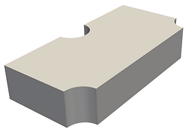
The final control geometry can be seen in the figure below for both the solid (left) and fluid (right).

MESHING
SnappyHexMesh (sHM) was selected for the meshing stage of the project. Investigation into the available online resources confirmed the decision that snappyHexMesh was the most appropriate meshing tool for the investigation.
The sHM tool builds on the basic mesh created by blockMesh, the first level meshing tool required within every OpenFOAM simulation. BlockMesh creates a bounding box for the geometry, and specifies the resolution and grading required for the initial hexahedral mesh. It is also used for the specification of patch types within some simulations. Within the sHM dictionary there are three main sub-dictionaries; castellation, snapping, and layers.
A medium quality mesh showing an increasing expansion ratio further away from the solid/ fluid interface is shown below.

SOLVING
The solving area of the research, involving the creation, editing and running of the simulation cases, was undertaken by several team members due its high labour intensity.
The simulation of the heat exchanger required that both fluid and solid regions be modelled, and the interaction between them be observed. The most appropriate solver for this application is chtMultiRegionFoam, a transient solver used in conjugate heat transfer cases.
Due to the complexity of the solver, the simulation was built up in stages. First a two-block case was analysed consisting of a solid block and fluid block. Then a three-block case with an additional solid block was simulated. After that, a three block with pin simulation was carried out. Working up to the final geometry and simulation setting. This process can be viewed in the Project Updates section of the website.
The final required subdirectories within the 0, constant and system folders that were set-up in this project are displayed below.


